Due: Your report must be submitted by 9:30 a.m. on Tuesday, December 5.

Group project: Your group is limited to at most four members. Once a group begins work on the project, its membership cannot change. Consequently establishing your group must be your first step in this project. Each group will submit one report, and all members of the group will receive the same grade for this project.

Goals:

1. To become familiar with the long-term behavior of solutions to certain forced second-order equations.
2. To study the relationship between the frequency of the forcing and the amplitude of the solutions.

Second-order equations: Using all of the methods that we have developed in this course, you will analyze the long-term behavior of the solutions to two similar forced, second-order equations.

We begin with the forced harmonic oscillator

Here b is the damping coefficient, k₁ is the spring constant, and w determines the frequency of the forcing.

1. (An undamped, forced linear equation) First consider the equation in the case where b=0. Using the Method of the Lucky Guess, determine a particular solution to the equation. Then using a numerical solver and/or the formulae for the solutions, estimate the amplitudes of the solutions for frequencies w in the interval 0 <= w <= 5. How do the amplitudes in the nonresonant case relate to the amplitudes in the resonant case?

2. (Damped, forced linear equations) Assume that the forcing is present along with some damping (b>0). How long does it take any given solution to get close to the steady-state solution? Using a numerical solver and/or the formulae for the solutions, estimate the maximum amplitudes of the solutions for frequencies w in the interval 0 <= w <= 5 for various values of b. Graph the maximum amplitude as a function of frequency for different values of b, all on the same set of axes. What happens to these graphs as b -> 0?

Now we return to the mass-spring system with a rubber band that we studied in the first project. Recall that the differential equation for that autonomous (unforced) system is

(see Project #1 for an explanation of the notation).

We will use this differential equation as a (very simplified) model of the Tacoma Narrows Bridge (see Section 4.5 in our text). Pictures of the current bridge and movies of the collapse of the original Tacoma Narrows Bridge, Galloping Gertie, are available on the web from the Washington State government and the College of Engineering at Iowa State University.

We now introduce a term of the form A sin wt to model a periodic external force, presumably caused by the wind in Tacoma Narrows, and we obtain the forced equation

For the remainder of this project, we will assume that b=0.01, A=0.1, and w=4.

3. (small amplitude periodic solution) Using analytic techniques as in Part 1, calculate a periodic solution that has small amplitude, and use a numerical differential equations solver to verify your calculation. Provide illustrations of its y(t)-graph and its solution curve in the phase plane. What are the initial conditions for this solution?

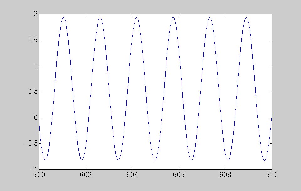
4. (large amplitude periodic solution) This system also has a large amplitude periodic solution that "attracts" many other solutions just as the small amplitude periodic solution attracts many solutions.

   The graph at the left is the graph of the large amplitude periodic solution for values of k1 and k2 that are close to (but not the same as) the values that you are using.

   Use a numerical solver to find this solution and provide illustrations of its y(t)-graph and its solution curve in the phase plane. What are its initial conditions? Describe the process that you used to locate the large amplitude periodic solution.

   Please note: This part of the project is difficult because it takes a long time (often 1000 units of time) for typical solutions to settle down to either the small amplitude solution or the large amplitude solution. In addition, it is difficult to find initial conditions that lead to the large amplitude solution without doing a little bit of programming.

   I found the initial conditions for the large amplitude solution graphed above by taking a modest sized grid of initial conditions in the 0 <= y <= 5 and 0 <= y' <= 5 square in the phase plane, and then I used MATLAB's ode45 to produce an approximate solution for each initial condition. The results can best be expressed in the form of the figure such as:

   

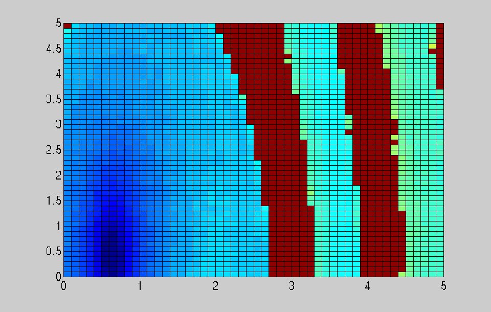
   The blue grid points represent initial conditions that produced solutions that are eventually asymptotic to the small amplitude solution. The red grid points represent initial conditions that came nowhere near the the small amplitude solution for 0<=t<=1000.

   It is a little tricky to use a computer to tell if you have found a periodic solution, but for this equation you can take advantage of the fact that the equation is periodic in t with period pi/2. So if a solution goes for pi/2 units of time and ends up back at the same initial condition, then the solution has to be periodic. (Why? This point of view is discussed on pp.477-484 of our text.)

   It took 10 hours of computer time for me to generate the grid shown above, and I do not really expect you to be able to produce such a figure for your equation. (However, it would be very impressed if you did.) In any case, just thinking about what that figure says should help you come up with a strategy for locating the large amplitude periodic solution.

Your report: Your report should be no longer than five typewritten pages, and it should address all of the questions mentioned above. You may provide as many illustrations from the computer as you wish, but the relevance of each illustration to your report must be evident. Illustrations are not included in the five-page limit. (Please remember that, although one good illustration may be worth 1000 words, 1000 illustrations are worth nothing.) Please insert your illustrations at appropriate places in your report rather than attaching them to the end of the report. Examples of good reports done here at BU in previous semesters are available for inspection in my office.

Numerical simulation: Be aware of the fact that pplane cannot handle nonautonomous systems. Therefore, you must use one of MATLAB's built-in ode solvers when you analyze the solutions to these equations numerically. Note my FAQ answer regarding the format of MATLAB files that define systems of differential equations.

Parameter values: The values of k₁ and k₂ that you should use are determined by the last digits of the BU ID numbers of the members of your group. Use k₁ = 12 + 0.1 a and k₂ = 5 - 0.05 a where a is the average (accurate to two decimal places) of the last digits of all members in the group. For example, if the last digits are 0, 1, 2, and 2, then a = 1.25, k₁ = 12.12, and k₂ = 4.94.

Academic Conduct: Your work and conduct in this course are governed by the CAS Academic Conduct Code. This code is designed to promote high standards of academic honesty and integrity as well as fairness. Copies of the code are available in CAS Room 105, and it is your responsibility to know and follow the provisions of that code. In particular, all work that you submit in this course must be your original work. For example, the computations that you do for your report as well as the text of your report must be original to your group. All group members are responsible for all aspects of the report. Any cases of suspected academic misconduct will be referred to the CAS Student Academic Conduct Committee.